The following tutorial teaches you how to analyze the data in your inventory using Excel 2007. Note: Excel 2007 differs somewhat from previous versions of the program; another tutorial on this website teaches you to analyze inventory data using Excel 2003.

We recommend using Excel for maintaining and updating the inventory because it is easy to use and generally familiar to most computer users, and it can also be used to analyze inventory data.

There are a number of ways to get inventory data into Excel. How you choose to get the data into Excel depends in large measure on how the data was collected.

(1) If your data was collected using a paper form, it will need to be entered manually into Excel; manual entry is time consuming, especially when the inventory involves large numbers of trees.

(2) If your data was collected using the STRATUM/MCTI PDA Utility, it will be in an Access mdb file format and can be imported from the STRATUM_MCTI_Inventory table in the Access i-Tree_Grand_Database.mdb file as follows:

• Office Button > Open
• Navigate to location of the inventory i-Tree_Grand_Database.mdb file
• Make sure that "Files of type" is set to "Access Databases"
• Import the inventory i-Tree_Grand_Database.mdb file

(3) If data is in the form of a GIS shapefile, it can be imported from the underlying dbf file as follows:

• Office Button > Open
• Navigate to location of the inventory shapefile
• Make sure that "Files of type" is set to "dBase files"
• Import the inventory dbf file

Note: data fields used in the examples below are based on the data fields in the Sample Tree Inventory Workbook and the Paper Survey Template. The data fields in your inventory may differ from the fields in this workbook and template.

Filtering Data - to find all records in the inventory possessing a common feature

Filter your tree inventory by field to generate a list based on a specified attribute. For example, you may wish to generate a list of all trees with a "Consult" designation, all available planting sites, all trees of a particular species, etc.

To filter the inventory data for all trees with a "Consult" designation in the Sample Tree Inventory Workbook:

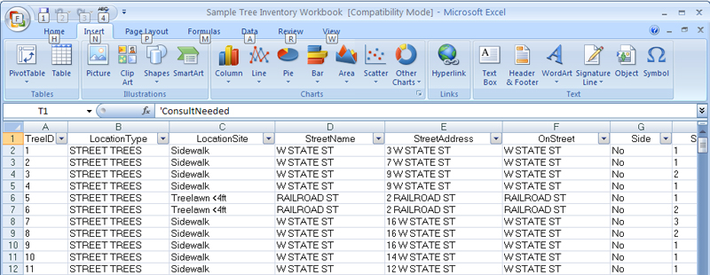
• Click on the Data tab at the top of the Excel spreadsheet (the All Sites worksheet tab at the bottom of the spreadsheet should be active)
• Click on Filter (below "View") - a downward pointing arrow should appear at the top of each column (see image below)

Larger image

• At the top of the ConsultNeeded column (you will probably need to scroll to the right in the spreadsheet to find this column), click on the arrow to expand the Pop-up menu - by default, all the boxes under "Text Filters" are checked
• Click on Select All to uncheck all the boxes
• Click on Yes so that it is checked
• Click on Okay at the bottom of the Pop-up menu
• A new list will be created showing only those records in the inventory where a consult designation of "Yes" was given
• To return all records to view, click on Clear (next to "Filter")

Inventory data can be filtered for multiple criteria. For example, suppose you wanted to generate a list of all trees with a "Consult" designation that are Sugar Maples with a dbh greater than or equal to 30. This can be done as follows:

• Repeat the steps above to generate a list of those records in the inventory where a consult designation of "Yes" was given
• At the top of the CommonName column, click on the arrow to expand the Pop-up menu - by default, all the boxes under "Text Filters" are checked
• Click on Select All to uncheck all the boxes
• Click on Sugar Maple so that it is checked
• Click on Okay at the bottom of the Pop-up menu
• A new list will be created showing only those records in the inventory where a consult designation of "Yes" was given that were also Sugar Maples
• At the top of the DBH column, click on the arrow to expand the Pop-up menu - by default, all the boxes under "Text Filters" are checked
• Highlight Number Filters in the Pop-up menu - a new Pop-up menu will appear to the right
• Click on Greater Than Or Equal To
• In the Custom Auto Filter message box, enter 30 in the box beside "is greater than or equal to"
• Click on Okay at the bottom of the message box
• A new list will be created showing only those records in the inventory where a consult designation of "Yes" was given that were also Sugar Maples with a dbh greater than or equal to 30.

To save your new list as a new spreadsheet table:

• Click on the box with the diagonal arrow immediately above the first record in the first column on the left - this will highlight in blue the entire table
• Right click anywhere in the table
• Click on Copy in the Pop-up menu
• Click on an empty worksheet tab at the bottom of the spreadsheet (if you need to create a new worksheet, right click on any of the tabs, click on Insert in the Pop-up menu, click on Worksheet and Okay in the Insert message box)
• In the empty worksheet, click on cell 1A (column A row 1)
• Right click in this box
• Click on Paste in the Pop-up menu
• The list you created by filtering data will be copied to the worksheet

Making Pivot Tables - to summarize values within a data field

Create a pivot table to summarize and graph your data. For example, you can use a pivot table to analyze Species Distribution, Genus Distribution, Size Class Distribution, Tree Condition, Percent Stocking, etc.

To create a pivot table analyzing the species distribution for all trees in the Sample Tree Inventory Workbook:

• Click on the Insert tab at the top of the Excel spreadsheet (the All Sites worksheet tab at the bottom of the worksheet should be active)
• Click on PivotTable (extreme left, below the Office Button)
• In the Create Pivot Table message box, the default settings are to select all the records in the worksheet as the range and to place the Pivot Table in a new worksheet - if these settings are acceptable, click Okay at the bottom of the message box
• A new sheet will be created with a Pivot Table Tools menu appearing at the top of the spreadsheet
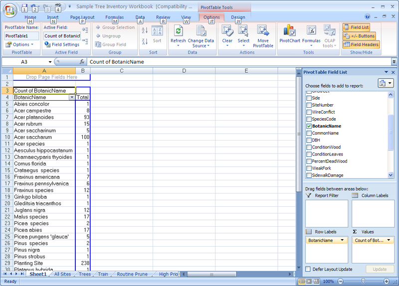
• On the right side of the spreadsheet, under Pivot Table Field List, click in the empty box next to Botanic Name
• Column A will be filled with a column listing all botanic names found in the worksheet and the Row Labels window at the bottom of the Pivot Table Field List will contain "Botanic Name"
• Place the cursor on "Botanic Name" in the Pivot Table Field List so that it is highlighted and drag "Botanic Name" into the ∑ Values window
• Column B will be filled with a count for the number of trees of each species found in the worksheet (see image below)

Larger image

• Right click on cell 3A: Count of Botanic Name
• In the Pop-up window, click on Summarize Data By - a new Pop-up menu will appear to the right
• Click on More Options at the bottom of the menu
• In the Value Field Settings message box, click on the Show values as tab
• Under "Show values as" click on the arrow to the right of "Normal" and click on % of total
• Click on Okay at the bottom of the message box
• Column B will be filled with a percentage for each species of the total number of trees found in the worksheet
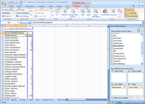
• To represent these percentages in a chart, click on Pivot Chart in the Pivot Tools Options menu at the top of the spreadsheet (if this menu is not visible, click anywhere in Count of Botanic Name table and the Pivot Tools Option tab will reappear)

The data in the Count of Botanic Name table can be filtered in much the same as the data in a worksheet:

• Click on the arrow in cell 4A to the right of Botanic Name
• In the Pop-up window, click on Value Filters -- a new Pop-up menu will appear to the right
• Click on Top 10
• In the Top 10 Filter message box, click on Okay
• The Count of Botanic Name table will now show the ten most prevalent species and the percentage for each species of the total number of trees of these ten species (not the total number of trees)
• To represent these percentages in a chart, click on Pivot Chart in the Pivot Tools Options menu at the top of the spreadsheet

You may have noticed that "Planting Site" is the most common species since planting sites are included in the All Sites worksheet. To filter out planting sites and obtain a more valid analysis of tree species:

• Click on the arrow in cell 4A to the right of Botanic Name
• In the Pop-up Window, scroll to Planting Site in the list of species immediately below "Value Filters"
• Click on the Planting Site box to uncheck it
• The table (and an associated graph if you have created one) will reflect the removal of "Planting Site" from inclusion in the table

Using STRATUM

Back to Conducting a Street Tree Inventory